AI SIMPLY EXPLAINED
All You Need To
Know About AI
Simply explained: Logistic Regression for Classification
Let us go over the basics and understand the need to introduce Logistic Regression.
Imagine you 're Dr. Alex, a dedicated oncologist at a renowned hospital. Your primary responsibility is to diagnose tumours as malignant (cancerous) or benign (not cancerous). To aid in this task, you 're given a software. Each time you input a tumour’s characteristics, the software promptly labels it either 'M ' (for malignant) or 'B ' (for benign). It feels almost like a superpower, but deep inside, you 're curious. How does this software classify the inputs and make such accurate predictions? Well, let us unveil its secret.

What is Classification?
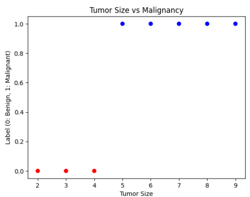
You recall your early days at med school where you had data on a bunch of tumours. Some were labeled 'M', and some were 'B'. You chart them on a graph, with the size of the tumour on the x-axis and the labels on the y-axis. There 's a clear pattern; larger tumours tend to be malignant while smaller ones tend to be benign. This is the essence of classification - to categorize data into classes based on certain features. In your case, you have two classes: malignant and benign, and you use the tumor 's size as the feature. Let us visualize an example dataset:

The Twist: Why Not Linear Regression?
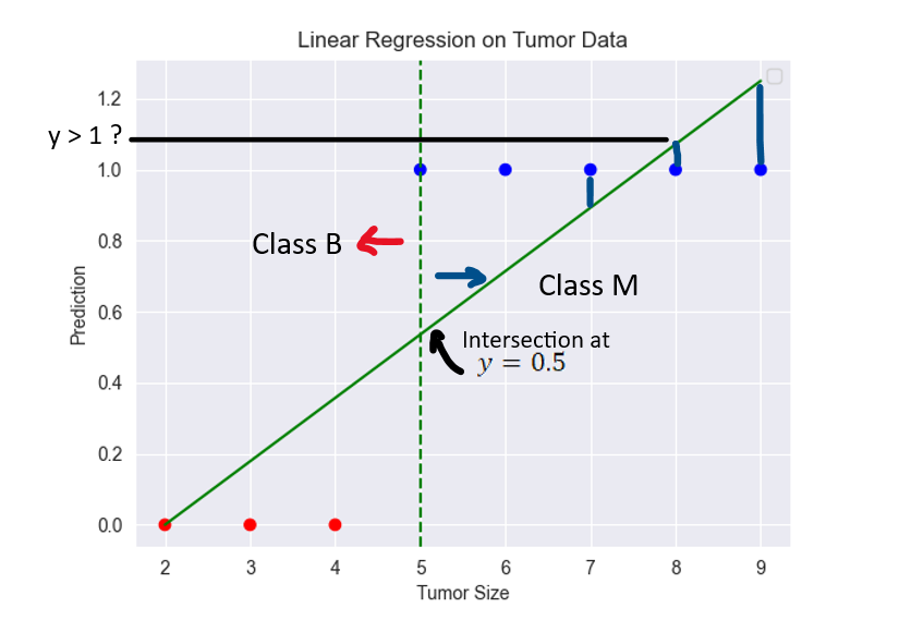
Using linear regression, a technique from statistics, to predict tumour malignancy seems perfect: and upon choosing a threshold value, let us say 0.5 one might classify a data point to be Class M if the predicted values are greater than the said threshold else Class B. However, upon trying it, the outliers skew the line in weird directions, making predictions inaccurate. Even worse, some predictions fall outside the 0-1 range, making no sense at all. The simplicity of a straight line is failing in the face of complex, real-world data. You realize you need a tool designed explicitly for classification tasks.
from sklearn.linear_model import LinearRegression

lin_reg = LinearRegression().fit(tumor_sizes.reshape(-1,1), y)
predictions = lin_reg.predict(tumor_sizes.reshape(-1,1))

Enter The Hero: Logistic Regression
Logistic Regression recognizes that predicting something like tumour malignancy isn 't about drawing straight lines but about understanding probabilities.
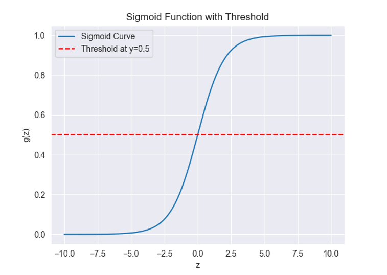
The magic behind logistic regression is the 'sigmoid function '. You 're probably wondering, "What makes the sigmoid function so special?" The sigmoid function gracefully handles outliers by squeezing any input into a value between 0 and 1, which is perfect for probabilities. It's shaped like an 'S ', starting near 0, increasing gradually, and then levelling off near 1.
The function is defined as:


We can then train the model on already labelled tumour size data and make predictions based on the model. Leveraging the scikit-learn library in Python, we can transform a few lines of code into a life-saving tool. Let us get into it then and use an example dataset where each row represents a tumour and has features like tumour size, age of the patient, etc and the target variable Malignant or Benign.
import numpy as np
import matplotlib.pyplot as plt
from sklearn.linear_model import LinearRegression
from sklearn.datasets import load_breast_cancer
from sklearn.model_selection import train_test_split
from sklearn.metrics import accuracy_score

# Load the dataset
data = load_breast_cancer()
X = data.data
y = data.target

# Split the data into training and test sets (70% train, 30% test)
X_train, X_test, y_train, y_test = train_test_split(X, y, test_size=0.3, random_state=42)

# Create a logistic regression model
model = LogisticRegression(max_iter=10000)  # increasing max_iter to ensure convergence

# Train the model
model.fit(X_train, y_train)

# Predict on the test set
y_pred = model.predict(X_test)
# Evaluate the accuracy of the model
accuracy = accuracy_score(y_test, y_pred)
print(accuracy)
Import all the necessary libraries and the preloaded breast_cancer dataset:
Think of the model as a wizard and the libraries as its helping elves:
- numpy was the alchemist, turning raw data into structured potions.
- LogisticRegression was the predictor, foretelling if a patient had cancer.
- train_test_split divided the labelled prophecies into those to learn from and those to test the predictor 's accuracy.
- accuracy_score was the judge, determining how well the predictor did its job.
Load the Dataset - the vault of knowledge X and y
X: This represents the feature matrix. Each row corresponds to a sample, and each column represents a feature.
y: This is the target variable or label. For logistic regression, it 's typically binary, representing two classes (0 or 1).
Split the data into training and testing sets (7:3)
The train_test_split function randomly divides the data into training and testing sets.
test_size=0.3 means that 30% of the data will be used for testing the predictors foresight, and the remaining 70% for training. This division ensures that the predictor was not biased by knowing all the answers beforehand.
random_state=42 is a seed for the random number generator. Using a seed ensures reproducibility: you 'll get the same train/test split every time you run the code.
Create a logistic regression model and train the model
Once split, the LogisticRegression predictor began its training. Like a young wizard learning spells, it used the training knowledge to understand the signs and symptoms that often led to cancer. It practiced and honed its skills, through multiple iterations until it felt confident in its predictions (max_iter).
model.fit(X_train, y_train): Trains the model on the training knowledge. The wizard will learn the importance for the features in X_train to predict the labels in y_train.

Predict on the test set
With its newfound knowledge, the predictor then tried to foresee the outcomes of the remaining 30% of the cases, the ones it hadn 't seen during its training. It was time for a test, like venturing out in the real world for the first time.
Evaluate the model's accuracy
The accuracy_score function computes the accuracy of the model 's predictions (y_pred) against the true labels (y_test), accuracy of the predictor's prophecies against the real outcomes.
In the case of the tumors, the function examines the size and assigns it a probability. If the sigmoid function outputs 0.8 for a particular tumor, that means there 's an 80% chance it 's malignant. The beauty lies in its flexibility. No matter how bizarre the tumor data, the sigmoid function remains unshaken, always providing a sensible probability.
Thanks to logistic regression and its trusty sidekick, the sigmoid function, you 're better equipped to make life-saving decisions.
Inspired from Andrew Ng 's Machine Learning Specialization, Supervised Machine Learning: Regression and Classification, Coursera